Top

User Research Doesn’t Prove Anything

User Dialogues

Creating exceptional user experiences through research

A column by Steve Baty
March 20, 2007

Recently, I was reading through a sample chapter of a soon-to-be-published book. The book and author shall remain nameless, as shall the book’s topic. However, I was disappointed to read, in what otherwise appeared at first glance to be an interesting publication, a very general, sweeping statement to the effect that qualitative research doesn’t prove anything and, if you want proof, you should perform quantitative research. The author’s basic assumption was that qualitative research can’t prove anything, as it is based on small sample sizes, but quantitative research, using large sample sizes, does provide proof.

This may come as a shock to everyone, but quantitative research does not provide proof of anything either.

Here, I’m using the word proof in the mathematical sense, because that is the context within which the author made those statements. In mathematics, a proof is a demonstration that, given certain axioms, some statement of interest is necessarily true. The important distinction here is the use of the word necessarily. In user research, as with all avenues of statistical inquiry, we’re able to demonstrate only that a hypothesis is probably true—or untrue—with some specific degree of certainty.

Granted, I’m being pedantic; and you might think this just an interesting exercise in semantics. But let me take you through a brief survey of this topic, then perhaps you’ll appreciate the importance of this distinction.

Champion Advertisement
Continue Reading…

Statistical Sampling

In general, our user research activities involve working with a small subset of our overall audience of users, to

  • gather information about a particular topic
  • test users’ response to some feature of our design solution
  • measure an increase or decrease in the efficiency of performing a certain task
  • or some other similar goal

The size of the entire audience prohibits us from involving all of our users in our research activities.

Our first step is to select our sample from the total population of users. If we’ve done that successfully, our sample should reflect, as closely as possible, the composition of the full user population in the user characteristics that matter for our research.

For example, let’s say that we’re measuring the completion times for a set of tasks in a Web application. We should first think about the user characteristics that might make someone more or less able to complete the tasks. These characteristics might include manual dexterity—for mouse control—visual acuity or impairment, language comprehension skills, etcetera. We’re less interested in whether users are left-handed or right-handed, male or female. So when selecting our sample, we need to ensure that it represents the proportion of users with vision impairments, for example, rather than left-handedness. We refer to this attribute of the sample as its representation of the user population. In other words, our sample should be representative of the entire population.

There are a few other things we need to consider. All members of our overall user population should have an equally likely chance of our selecting them for our sample. This factor of sampling is known as randomness. So-called convenience samples—where we choose participants based on the fact that they’re close to us—obviously limit the likelihood of non-proximal users participating in our study, so don’t satisfy the requirement for randomness.

Lastly, our sampling technique should ensure that selecting one person has no affect on the chance that we’ll select another person. This factor is known as independence and is the same principle that describes the probability that a coin toss will result in a head or tail showing. The chance of getting a head on a single coin toss is half, or 50%. The chance that two heads will appear in a row is ½ x ½ = ¼. However, if our first coin toss shows a head, the chance that the second toss will show a head is back to being half, because the two events—our two coin tosses—are independent of one another. (Bear this in mind the next time you see a run of five black on a roulette table. You might hear someone say, “The next one must be red; the chances of having six black in a row are really low.” But really, the odds are fifty-fifty that the next one will be black.)

So, once we have selected a random, independent, representative sample, we carefully conduct our user research—survey, usability testing, etcetera—then measure our test results.
Inferential Statistics

There are two things we can do with our data:

  • Calculate summary or descriptive measures.
  • Use our sample statistics to estimate the values of those measures for the user population as a whole.

First, we usually calculate summary or descriptive measures such as

  • the arithmetic mean—what we commonly call the average
  • the mode—the most commonly measured value
  • the median—the middle value when we rank all measures

We also might measure the variance in a summary or descriptive measure—and a host of other values we can calculate from our sample. We collectively refer to these as sample statistics.

The mistake that researchers often make is to stop at this point and start talking as if we now have learned something definite about our user population as a whole. Statements such as the following are all complete nonsense:

  • “78% of users think…”
  • “85% of teenagers on MySpace believe…”
  • “The majority of users will…”

The simple words “Of the users who completed the task/survey question/etcetera…” should preface all such statements.

Of course, I said there were two things we can do with our data. The second is to use our sample statistics to estimate the values of those same measures—mean, variance, etcetera—for the user population as a whole. We do this, because, in most cases, our intent is to learn something about our entire user population.

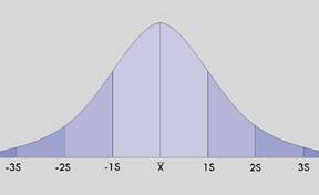
It is a remarkably simple process to make this jump from a sample to an entire user population. The key thing to understand, in taking this step, is that, if we took a second sample and measured the same values—mean, variance, etcetera—we’d expect to get numbers that were close to, but not exactly the same as our first sample. In fact, if we were to repeat this process over and over, the values we measured for the mean and variance would form a standard bell-shaped curve like that shown in Figure 1—called variously the normal distribution or Gaussian distribution—after the 19th century German mathematician who used it so extensively in his work on astronomy.

Figure 1—A bell-shaped curve
Bell-shaped curve

This characteristic of sample statistics provides us with the means by which we can estimate statistics for an entire user population from a single sample. We can use the sample mean directly—as an estimate for the population mean. Because the sample means form a normal distribution, we know that the actual population mean will fall within a plus or minus range around our sample mean. That plus or minus range is based on the variance in the sample. When using the sample variance to estimate the population mean, we first transform it into a standard error, using the formula:

Formula

where s is the standard deviation for the sample—that is, the square root of the variance—and n is the number of users in our sample.

Based on our sample mean, we can be 95% certain that our actual population mean will sit within the range x ± 2se, where x is the sample mean—to be precise, the actual range is x ± 1.96se for a 95% range. We can be 99.7% certain that the actual population mean will sit within the range x ± 3se.

Note that, in each case, there exists a small chance that the actual population mean will fall outside the range that we’ve defined. This chance is why I referred earlier to the distinction between something probably being true and something necessarily being true.

Also, our standard error (se) is a function of the number of users in our sample. The more people we sample, the smaller the value of se and the narrower the range we define for our population mean. However, because we use the number of sample users as a square root, to halve our estimated range, we need to sample four times as many users. This is why people tend to say that quantitative studies require more users than qualitative studies. Because we’re trying to minimize the range of our estimate, we want to minimize the value of the standard error.

The techniques I’ve described work for all measured values—for example, task completion times—and allow you to start making more meaningful statements about your user research data. In the absence of such techniques, the conclusions you draw from your research lack adequate foundation, and those reviewing your reports can easily reject them. More importantly, the efforts you expend in conducting your research will be largely wasted for want of some simple analytical rigor.

The estimated range we can provide for the population mean gives us a reasonable likelihood—95%, say—that the real population mean will actually fall within the bounds of that range. However, not only have we been unable to pinpoint exactly the population mean, there still exists a slight chance—5% in this example—that the actual value will fall outside this range. More importantly, that uncertainty exists regardless of the number of users we include in our test. All we can do is narrow the range and, in so doing, get closer to the real value for the entire user population. So quantitative studies, while providing us with a method for estimating user population statistics, cannot provide us with proof. Used carefully, however, they can tell us a great deal—and if not with certainty, at least with a known amount of uncertainty. 

Co-founder & Principal at Meld Studios

Sydney, New South Wales, Australia

Steve BatyFocusing on the business side of the user experience equation, Steve has over 14 years of experience as a UX design and strategy practitioner, working on Web sites and Web applications. Leading teams of user experience designers, information architects, interaction designers, and usability specialists, Steve integrates user and business imperatives into balanced user experience strategies for corporate, not-for-profit, and government clients. He holds Masters degrees in Electronic Commerce and Business Administration from Australia’s Macquarie University (MGSM), and a strong focus on defining and meeting business objectives carries through all his work. He also holds a Bachelor of Science in Applied Statistics, which provides a strong analytical foundation that he further developed through his studies in archaeology. Steve is VP of the Interaction Design Association (IxDA), a member of IA Institute and UPA, founder of the UX Book Club initiative, Co-Chair of of UX Australia, and an editor and contributor for Johnny Holland.  Read More

Other Columns by Steve Baty

Other Articles on User Research

New on UXmatters